Functions

In this “chapter” I will attempt to run through some required function knowledge for calculus.

What is a function?

The natural world is full of relationships between quantities that change. When we see these relationships, it is natural for us to ask “If I know one quantity, can I then determine the other?” This establishes the idea of an input quantity, or independent variable, and a corresponding output quantity, or dependent variable. From this we get the notion of a functional relationship in which the output can be determined from the input.

For some quantities, like height and age, there are certainly relationships between these quantities. Given a specific person and any age, it is easy enough to determine their height, but if we tried to reverse that relationship and determine height from a given age, that would be problematic, since most people maintain the same height for many years.

Definition of a Function

A function is rule for a relationship between an input, or independent, quantity and an output, or dependent, quantity in which each input value uniquely determines one output value. We say “the output is a function of the input.”

Following are some things to consider: * In the height and age example above, is height a function of age? Is age a function of height? * In the height and age example above, it would be correct to say that height is a function of age, since each age uniquely determines a height. For example, on my 18th birthday, I had exactly one height of 69 inches. * However, age is not a function of height, since one height input might correspond with more than one output age. For example, for an input height of 70 inches, there is more than one output of age since I was 70 inches at the age of 20 and 21.

Function Notation

To simplify writing out expressions and equations involving functions, a simplified notation is often used. We also use descriptive variables to help us remember the meaning of the quantities in the problem.

Rather than write “height is a function of age,” we could use the descriptive variable h to represent height and we could use the descriptive variable a to represent age.

---

Example

“Height is a function of age”. If we name the function \(f\) we write “\(h\text{ is }f\text{ of }a\)”, or more simply \(h=f(a)\). We could instead name the function \(h\) and write \(h(a)\) which is read “\(h\) of \(a\)”.

---

Remember we can use any variable to name the function; the notation \(h(a)\) shows us that \(h\) depends on \(a\). The value “\(a\)” must be put into the function “\(h\)” to get a result. Be careful – the parentheses indicate that age is input into the function (Note: do not confuse these parentheses with multiplication!).

The notation output = \(f(\text{input})\) defines a function name \(f\). This would be read “output is \(f\) of input”.

---

Example

A function \(N=f(y)\) give the number of police officers, \(N\), in a town for year \(y\). what does \(f(2022)=300\) tell us?

Solution

When we read \(f(2022)=300\), we see the input quantity is \(2022\), which is a value for the input quantity of the function, the year, \(y\). The output value is \(300\), the number of police officers, \(N\), a value for the output quantity. Remember \(N=f(y)\). So this tells us that in the year \(2022\) there were \(300\) police officers in the town.

---

Table of Values

Functions can be represented in many ways: Words (as we did in the last few examples), tables of values, graphs, or formulas. Represented as a table, we are presented with a list of input and output values.

This table represents the age of children in years and their corresponding heights. While some tables show all the information we know about a function, this particular table represents just some of the data available for height and ages of children.

Solving and Evaluating Functions

When we work with functions, there are two typical things we do: evaluate and solve. Evaluating a function is what we do when we know an input, and use the function to determine the corresponding output. Evaluating will always produce one result, since each input of a function corresponds to exactly one output.

Solving equations involving a function is what we do when we know an output, and use the function to determine the inputs that would produce that output. Solving a function could produce more than one solution, since different inputs can produce the same output.

---

Example

Using the table shown, where \(Q=g(n)\)

\(n\)	\(Q\)
1	8
2	6
3	7
4	6
5	8

Table of values for \(Q=g(n)\).

1. Evaluate \(g(3)\).

2. Solve \(g(n)=6\).

Solution

For (a) it is important to realize we want to input \(3\) into the function \(g\) to find the output. Whereas for (b) we want to find the input such that the output is \(6\). These are important distinctions for future conversations.

1. Evaluate \(g(3)\): Evaluating \(g(3)\) (read: “ g of 3” ) means that we need to determine the output value, \(Q\), of the function \(g\) given the input value of \(n=3\). Looking at the table, we see the output corresponding to \(n=3\) is \(Q=7\), allowing us to conclude \(g(3)=7\)..

2. Solve \(g(n)=6\): Solving \(g(n)=6\) means we need to determine what input values, \(n\), produce an output value of \(6\). Looking at the table we see there are two solutions: \(n=2\) and \(n=4\). When we input \(2\) into the function \(g\), our output is \(Q=6\). When we input \(4\) into the function \(g\), our output is also \(Q=6\).

---

Functions and Graphs

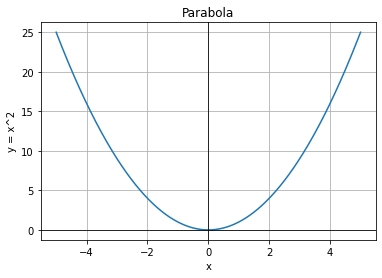
Oftentimes a graph of a relationship can be used to define a function. By convention, graphs are typically created with the input quantity along the horizontal axis and the output quantity along the vertical.

import matplotlib.pyplot as plt
import numpy as np

x = np.linspace(-5, 5, 400)
y = x**2

plt.figure()
plt.plot(x, y)
plt.title('Parabola')
plt.xlabel('x')
plt.ylabel('y = x^2')
plt.grid()
plt.axhline(0, color='black', linewidth=0.8)  # Add horizontal axis
plt.axvline(0, color='black', linewidth=0.8)  # Add vertical axis
plt.show()

theta = np.linspace(0, 2*np.pi, 400)
r = 2

x = r * np.cos(theta)
y = r * np.sin(theta)

plt.figure()
plt.plot(x, y)
plt.title('Circle')
plt.xlabel('x')
plt.ylabel('y')
plt.grid()
plt.axhline(0, color='black', linewidth=0.8)  # Add horizontal axis
plt.axvline(0, color='black', linewidth=0.8)  # Add vertical axis
plt.show()

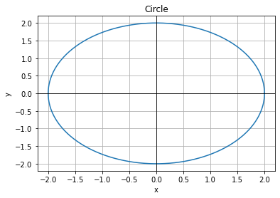
Looking at the two graphs above, the first define a function \(y=f(x)\), since for each input value along the horizontal axis there is exactly one output value corresponding, determined by the y-value of the graph. The second graph does not define a function \(y=f(x)\) since some input values, such as \(x=1\), correspond with more than one output value.

The vertical line test is a handy way to think about whether a graph defines the vertical output as a function of the horizontal input. Imagine drawing vertical lines through the graph. If any vertical line would cross the graph more than once, then the graph does not define only one vertical output for each horizontal input.

Evaluating a function using a graph requires taking the given input and using the graph to look up the corresponding output. Solving a function equation using a graph requires taking the given output and looking on the graph to determine the corresponding input.

import numpy as np
import matplotlib.pyplot as plt

# Define the equation
def equation(x):
    return (x - 1)**2

# Generate x values
x = np.linspace(-1.23606797749979,3.23606797749979, 400)

# Calculate y values using the equation
y = equation(x)

# Set up the figure and plot
plt.figure()
plt.plot(x, y, label='$y = (x - 1)^2$')
plt.title('Plot of $y = (x - 1)^2$')
plt.xlabel('x')
plt.ylabel('y')
plt.grid(True, linestyle='--', linewidth=0.8)
plt.axhline(0, color='black', linewidth=0.8)
plt.axvline(0, color='black', linewidth=0.8)

# Set custom grid intervals
x_grid = np.arange(-5, 6)
y_grid = np.arange(-5, 6)
plt.xticks(x_grid)
plt.yticks(y_grid)

plt.legend()
plt.show()

Example

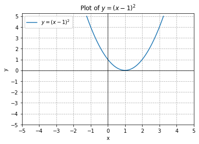
From the plot above: 1. Evaluate \(f(2)\). 2. Solve \(f(x)=4\).

Do this by only looking at the graph and they try doing it algebraically.

Solution

1. To evaluate \(f(2)\), we find the input of \(x=2\) on the horizontal axis. Moving up to the graph gives the point \((2,1)\), giving an output of \(y=1\). So \(f(2)=1\).

2. To solve \(f(x)=4\), we find the value \(4\) on the vertical axis because if \(f(x)=4\) then \(4\) is the output. Moving horizontally across the graph gives two points with the output of \(4\): \((-1,4)\) and \((3,4)\). These give the two solutions to \(f(x)=4\): \(x=-1\) or \(x=3\). This means \(f(-1)=4\) and \(f(3)=4\), or when the input is \(-1\) or \(3\), the output is \(4\).